
One click on “Refresh schema”, and after 60 seconds the browser shows the error message 504 Gateway Timeout, because the web server in front of the application will not wait any longer for a response. On the server, the work continues undisturbed, only nobody can see it. So a second click follows, then a third, and shortly afterwards four runs are computing at the same time. A single run across 1,000 tables took a measured 114 seconds. The requirement was less than three seconds.
The cause was not a slow query but a loop that asked the source database for each table individually and stored the result individually. This article describes how that loop was measured and replaced with set-based statements, that is, statements that read and write all 1,000 tables at once, and which options were weighed against each other. It also describes what went wrong along the way. The first of those statements was slower than 1,000 single queries combined, and the finished result missed its targets despite a gain by a factor of 9 to 19.
The essentials up front:
- A loop in application code costs more per iteration than the same loop inside the database: Whoever processes tables one at a time instead of with one statement over all of them pays a fixed overhead for every iteration, no matter how little data the iteration moves. If the loop lives in application code and opens its own database connection for each table, connection setup, authentication and a transaction are added per iteration. In the case described, one iteration cost around 114 milliseconds, which for all 1,000 tables adds up to the 114 seconds mentioned at the start. The same loop, rebuilt for this article as a procedure inside Postgres, cost around three milliseconds per table and thus around three seconds for the same 1,000 tables.
- The loop was not carelessness, and its strengths had to be rebuilt: For each table it called a function that already existed for activating a single table and that worked correctly there. If one table failed, the others carried on, and even four concurrent runs left no contradictory data behind. With the 15 to 70 tables that the real databases of this application have, the runtime never stood out. The solution that processes all tables at once had to restore this error isolation explicitly.
- One statement over all tables is not automatically faster than a thousand single ones: The first query that read the keys of all 1,000 tables at once from
information_schema, the views in which Postgres exposes its own metadata, took around five seconds on Postgres 17. Issued once per table instead, the same query adds up to an extrapolated half a second. The execution plan showed why: Postgres 17 had chosen a plan for this query that re-evaluated one of the two views involved for every table, and so it had rebuilt the loop internally. A query directly on the system tables inpg_catalogbehind those views took milliseconds, but it also showed every database user the keys of tables they are not allowed to read, and therefore needed a condition of its own for access privileges. - 114 seconds became 12, and the targets were still missed: Those twelve seconds apply to a run that rewrites all 1,000 tables. The more common case is a run over an unchanged set of tables, and for that one the target was three seconds, which allows three milliseconds per table. The new logic takes around 3.7 milliseconds per table and is thus just under a quarter over budget. Across 1,000 tables that is 3.7 seconds. The run still takes up to 6.4 seconds. The target was missed somewhere else, because the missing 2.7 seconds are what every call on the shared server costs before it touches the first table, among other things for authentication, permission checks and reading the table selection. Next to 114 seconds of loop, this share had never stood out, and the estimate before the rebuild did not include it.
Prerequisite: Basic SQL and an idea of what a stored procedure is. The examples are PL/pgSQL and were run on Postgres 17 and 18 in throwaway containers. The case described comes from an application written in TypeScript, whose code is not shown here because the mechanics do not depend on the programming language.
Contents
- The Starting Point: A Schema Snapshot Across 1,000 Tables
- Measuring Runtime When the Web Server Times Out
- Where the 114 Seconds Went
- The Same Loop Inside the Database
- What Spoke for the Loop
- What Spoke Against the Loop and What the Switch Costs
- The Decision: Four Options and a Budget Calculation
- Set-Based Is Not Automatically Fast: Why a Query Over All Tables Can Be Slower
- The Privilege Trap When Switching to pg_catalog
- The Result: Factor 9 to 19, Targets Still Missed
- When an Optimization Changes What a Display Means
- What Remains
- FAQ
- Related Articles
The Starting Point: A Schema Snapshot Across 1,000 Tables
The private project DI² generates ETL pipelines from the metadata of a source database. To know what it is working with, it reads the columns, the primary and unique keys and the foreign keys of every activated table and stores them as a snapshot in its own database. A click on “Refresh schema” repeats this read for all tables of a connection.
This refresh was implemented as a loop. For each table, the application code called a function that already existed. It read the metadata of a single table from the source and replaced that table’s snapshot in one transaction by deleting the old rows and inserting the new ones. The function had been written for a different occasion, activating a single table, and for that occasion it was correct. The loop on top of it was the obvious next step.
The specification had carried a target for the refresh for months: less than three seconds for 1,000 tables. Nobody had measured it, because the real databases in the project had between 15 and 70 tables. The measurement was made up for with a synthetic source database of 1,000 tables with 50 columns each. The tables were empty, because the refresh reads only the catalog, that is, the views and system tables in which Postgres describes which tables, columns and keys exist. The measurement ran on the project’s development server, a shared machine with four virtual cores and 7.6 gigabytes of memory.
Measurement, code analysis and rebuild were done with a coding agent, which had also written the application code. The trade-offs and decisions this article tells about were made by the maintainer. What that division of labor looks like day to day is described in the article Agentic Coding from a User’s Perspective.
The result of the measurement:
| Metric | Value |
|---|---|
| Duration of the loop, single run without concurrent runs | 114.4 s |
| Difference between two runs | 6 ms |
| Duration per table | around 114 ms |
| Reading the table list, the only set-based step | 22 to 43 ms |
| Target | under 3 s, missed by a factor of 38 |
None of this result reached the browser. The web server in front of the application ended the request after 60 seconds with a gateway timeout while the loop kept running on the server. Whoever clicked again started a second run next to the first. In the measurement session, up to four loops were running at the same time this way, and one of them delivered its response only after about seven minutes.
Measuring Runtime When the Web Server Times Out
Because the timeout cut off every measurement in the browser, the duration had to come from the data itself. The refresh replaces the snapshot of every table, and every newly written row receives a timestamp in created_on. After a run without concurrent runs, the span between the first and the last written row therefore gives the duration of the loop to within about one iteration, because the timestamp records the start of an iteration and not its end. The query for it needs no instrumentation at all:
  1: SELECT
  2:     count(DISTINCT table_name)        AS table_count
  3:    ,min(created_on)                   AS first_row
  4:    ,max(created_on)                   AS last_row
  5:    ,max(created_on) - min(created_on) AS duration
  6: FROM
  7:    meta.column_snapshot
  8: WHERE
  9:    schema_name = 'perf';
This calculation has a prerequisite that is easy to overlook. A default such as now() returns in Postgres the moment the current transaction began, not the moment of the insert. In the case study, every table ran in its own transaction, so every table got its own timestamp. If a procedure instead writes all tables in a single transaction, every row carries the same value, and the span is zero. A rebuild of the loop as a Postgres procedure, shown in the section “The Same Loop Inside the Database”, confirmed exactly that. With one COMMIT per table, the query returned the duration of the loop, 5 milliseconds less than the stopwatch on the call, which is the last iteration, whose end no timestamp records anymore. Without COMMIT it returned 00:00:00. Whoever needs the moment of every single row sets clock_timestamp() as the default. statement_timestamp() does not help here, because it returns the start of the statement the client sent, and for the whole procedure that is the CALL.
Two independent runs came to 114.439 and 114.445 seconds and were thus practically identical. A statement about the distribution would have needed more runs, but for finding the cause, the order of magnitude was enough. Since the rebuild, the application measures its own duration and writes it to the audit log, so the detour via the timestamps is no longer needed. That instrumentation was itself one of the consequences of the analysis. Why a query on the stored data often leads to a finding faster than clicking through the user interface is shown in the article The Agent Measures Where I Click.
Where the 114 Seconds Went
Per table, the following happened in sequence:
- Three connections to the source database: The code opened one connection each for columns, keys and foreign keys. Before each of these connections it loaded the connection profile from its own database and decrypted the password. Then it established a fresh TCP connection, authenticated, issued a single catalog query for exactly this table and closed the connection again. For 1,000 tables, that is 3,000 connection setups per refresh.
- Up to four procedure calls in its own database: One after the other, the column snapshot was replaced, the derived validation rules were reconciled, the key snapshot was replaced and the foreign-key snapshot was replaced.
The source database ran on the same machine, and the network between the containers costs less than a millisecond. The 114 milliseconds per table therefore consisted almost entirely of costs that every iteration pays regardless of the amount of data. How exactly they split between connection, profile and procedure calls, the measurement did not record. A separate measurement with pgbench between two containers gives the order of magnitude. There, one connection setup with password authentication cost 17 milliseconds on average, while a simple query over an existing connection cost 0.36 milliseconds. Postgres starts a separate server process for every new connection, and exactly this overhead was incurred three times per table in the loop. Three connection setups thus explain around 50 of the 114 milliseconds, and the rest is spread over loading and decrypting the profile and the four procedure calls.
The counter-evidence comes from the only step of the refresh that was already set-based, meaning it asked its question in a single statement for all tables instead of once per table. The list of all 1,000 tables came back in 22 to 43 milliseconds, which is less than 0.04 percent of the total time.
The target also yields a budget, and this calculation settles the question earlier than any optimization attempt. Three seconds for 1,000 tables come to three milliseconds per table. A single connection setup alone costs a multiple of that. As long as every iteration opens a connection, the target is therefore out of reach, no matter how fast the queries inside it are.
The Same Loop Inside the Database
The case study plays out in application code, but the pattern is the same as with a cursor in a procedure that works through a result set row by row. Among SQL developers it goes by the mocking name RBAR, short for “Row By Agonizing Row”. In the world of ORMs it is known as the N+1 problem: first one query for the list, then another one for every element. To see which part of the cost is tied to the loop itself and which to the connections, the snapshot was rebuilt inside Postgres for this article. It reads from information_schema, the standardized set of views through which most SQL databases describe their tables and columns. The target table takes one row per column:
  1: CREATE SCHEMA IF NOT EXISTS meta;
  2:
  3: CREATE TABLE meta.column_snapshot
  4: (
  5:     schema_name               text          NOT NULL
  6:    ,table_name                text          NOT NULL
  7:    ,column_name               text          NOT NULL
  8:    ,data_type                 text          NOT NULL
  9:    ,ordinal_position          int           NOT NULL
 10:    ,created_on                timestamptz   NOT NULL DEFAULT now()
 11:    ,created_by                text          NOT NULL DEFAULT current_user
 12:    ,PRIMARY KEY (schema_name, table_name, column_name)
 13: );
The sequential version reads the tables of a schema and writes each table’s snapshot in its own transaction, the way the case study did. The COMMIT inside the loop requires that the CALL is not inside an open transaction block:
  1: -- --------------------------------------------------------------------------------
  2: -- Parameters
  3: -- --------------------------------------------------------------------------------
  4: --    p_schema_name        text
  5: --       Schema whose tables are taken into the snapshot
  6: -- --------------------------------------------------------------------------------
  7: CREATE OR REPLACE PROCEDURE meta.sp_load_column_snapshot_loop
  8: (
  9:     IN    p_schema_name        text
 10: )
 11: LANGUAGE plpgsql
 12: AS $procedure$
 13: DECLARE
 14:    l_table_name              text;
 15: BEGIN
 16:
 17:    FOR l_table_name IN
 18:       SELECT
 19:          table_name
 20:       FROM
 21:          information_schema.tables
 22:       WHERE
 23:          table_schema = p_schema_name
 24:       ORDER BY
 25:          table_name
 26:    LOOP
 27:       -- --------------------------------------------------------------------------------
 28:       -- One table: delete the old snapshot, write the new one
 29:       -- --------------------------------------------------------------------------------
 30:       DELETE FROM
 31:          meta.column_snapshot
 32:       WHERE
 33:              schema_name = p_schema_name
 34:          AND table_name  = l_table_name;
 35:
 36:       INSERT INTO meta.column_snapshot
 37:       (
 38:           schema_name
 39:          ,table_name
 40:          ,column_name
 41:          ,data_type
 42:          ,ordinal_position
 43:       )
 44:       SELECT
 45:           table_schema
 46:          ,table_name
 47:          ,column_name
 48:          ,data_type
 49:          ,ordinal_position
 50:       FROM
 51:          information_schema.columns
 52:       WHERE
 53:              table_schema = p_schema_name
 54:          AND table_name   = l_table_name;
 55:
 56:       -- Each table is written in its own transaction
 57:       COMMIT;
 58:    END LOOP;
 59: END;
 60: $procedure$;
The lines in detail:
- Lines 17 to 54: The loop runs over the table list from
information_schema.tables, and for each table aDELETEand anINSERTfollow. That is the N+1 pattern: one query for the list, N more for the work. - Line 57: The
COMMITends the transaction after every table and thus rebuilds per-table atomicity. Without this line, the whole loop would run in a single transaction, and an error at table 500 would also roll back the 499 finished tables. The timestamp measurement from the previous section would then give zero, becausenow()returns the start of the transaction and stays constant within it. Procedures mayCOMMITsince Postgres 11, functions may not, and even a procedure may do so only as long as the caller holds no transaction open. If the caller opens one, for instance through a library that wraps every call inBEGINandCOMMIT, the procedure fails at the firstCOMMITwithinvalid transaction termination. What theCOMMITdoes not provide is the error isolation of the case study. This procedure has no error handling, and an error at table 500 ends the call. The 499 finished tables stay written, the remaining 500 stay unprocessed.
The set-based version does the job with two statements over the whole schema and therefore needs no loop. The difference sits in the WHERE clause: only the schema remains there, no longer the single table.
  1: -- --------------------------------------------------------------------------------
  2: -- Parameters
  3: -- --------------------------------------------------------------------------------
  4: --    p_schema_name        text
  5: --       Schema whose tables are taken into the snapshot
  6: -- --------------------------------------------------------------------------------
  7: CREATE OR REPLACE PROCEDURE meta.sp_load_column_snapshot
  8: (
  9:     IN    p_schema_name        text
 10: )
 11: LANGUAGE plpgsql
 12: AS $procedure$
 13: BEGIN
 14:
 15:    DELETE FROM
 16:       meta.column_snapshot
 17:    WHERE
 18:       schema_name = p_schema_name;
 19:
 20:    INSERT INTO meta.column_snapshot
 21:    (
 22:        schema_name
 23:       ,table_name
 24:       ,column_name
 25:       ,data_type
 26:       ,ordinal_position
 27:    )
 28:    SELECT
 29:        table_schema
 30:       ,table_name
 31:       ,column_name
 32:       ,data_type
 33:       ,ordinal_position
 34:    FROM
 35:       information_schema.columns
 36:    WHERE
 37:       table_schema = p_schema_name;
 38: END;
 39: $procedure$;
This also removes the COMMIT per table, because both statements run in the same transaction. In return, it gives up per-table atomicity: an error rolls back the whole run and not just the table being processed. The two versions have a second difference: the set-based one also deletes rows for tables that no longer exist, while the loop leaves them in place, because it only runs over the tables that are present.
On Postgres 18.6 in a Docker container on a laptop, the set-based version took around 0.6 seconds in three runs on a freshly created table, the loop around 3 seconds. Both versions wrote exactly the same 50,000 rows, and a comparison with EXCEPT ALL over the five business columns, that is, without the timestamps, showed no difference in either direction. On Postgres 17 the times varied more, and the ratio was similar. The laptop numbers serve as an order of magnitude, not as a benchmark, because with repeated overwriting without VACUUM both versions became noticeably slower.
A factor of five (3 seconds ÷ 0.6 seconds) is significant. It is still a long way from what the case study experienced, because there one iteration cost 114 milliseconds instead of three. The difference is made by the overhead that every iteration there paid on top of the actual work: three connection setups, three authentications, loading and decrypting the profile and four separate procedure calls. So a loop is not expensive simply because it is a loop. It becomes expensive in proportion to what an iteration costs beyond the work, and that share grows with every connection, every process and every transaction that sits between the loop and the data.
What Spoke for the Loop
Before the rebuild, the loop deserves a fair assessment, because it was not carelessness. Its advantages were real, and some of them the new solution had to rebuild explicitly.
- Reuse: The function for a single table already existed and was tested. A loop on top of it brought neither a new code path nor a new class of errors.
- Per-table error isolation: If table 738 fails because of a missing permission or a concurrent
DROP TABLE, the application code catches the error, increments an error counter, and the remaining 999 tables carry on. This property comes from the loop’s error handling and not from the transaction per table that the next point describes. - Per-table atomicity: Delete and re-insert ran in a transaction of their own for every table, so that even under concurrency no half snapshot of a single table ever came about. It does not guarantee a common state of all 1,000 tables from one and the same run, but the snapshot does not need that either, because every table is read on its own and used on its own. In the measurement session this proved itself: of seven runs, five overlapped, not one reported an error, and in the end exactly 50,000 rows for 1,000 tables were in place.
- Constant memory footprint: The application never held more than one table in memory.
- Readability: The control flow was an ordinary loop that anyone understands on first reading.
- Inconspicuous at small scale: A database with 48 tables would have taken an extrapolated five to six seconds. That is a noticeable wait, but not an alarming one.
The problem came with scale, not with the original decision.
What Spoke Against the Loop and What the Switch Costs
Four points spoke against the loop:
- Fixed cost times count: Connection, authentication, profile and procedure call are incurred in every iteration, while the actual amount of data per table is tiny. More than 99.9 percent of the runtime sat in the loop over the tables.
- The catalog answers set questions at almost the price of a single question: In the rebuild,
information_schema.columnsdelivered all 50,000 columns in around 0.3 seconds. The columns of a single table took 6 to 15 milliseconds as a query of their own, and repeated a thousand times that is 6 to 15 seconds. The largest part of that is planning the view query, on Postgres 18.6 around 5 milliseconds against around one millisecond of execution. In a PL/pgSQL procedure this planning does not happen on every iteration: the procedure creates a prepared statement on the first iteration and switches after a few iterations to a cached plan that does not depend on the concrete values, provided that plan is not much worse. That is why the loop in the rebuild gets by with around three milliseconds per table. With the settingplan_cache_mode = force_custom_plan, which re-plans on every iteration, the same loop took around two and a half to three seconds longer. - Set-based writing spreads the cost over many rows: In the same project, a single
INSERTinto a different table wrote around 91,000 rows in about one second, as an order of magnitude and not as a comparison under equal conditions. The loop moved less data with its 50,000 rows and took 114 seconds for it. - Collision with timeouts: A synchronous operation that takes longer than the timeout of the web server in front of it produces an error message behind which the work continues. Users click again, and the runs pile up.
The switch to set-based processing, however, has a price of its own:
- The batch size becomes a decision in its own right: A batch is a single call of a procedure that accepts the data of many tables at once, in the case described as a JSON document with all columns, keys and foreign keys of those tables. How many tables belong in it, someone has to decide, and before the switch the question did not arise at all. The amount of data per call has to fit the memory limits of the application and the parameter limits of the database drivers.
- Errors hit larger units: If a batch fails, that affects all tables in it. The per-table count has to be restored actively.
- Transactions take longer: A batch holds its locks longer than many small transactions do.
- More code has to be right at once: Each of the three supported engines, PostgreSQL, SQL Server and MySQL, needs its own set-based queries against its catalog. The new batch procedures are new objects with tests of their own.
- Equivalence has to be proven: The rebuild must not change the stored result, so a before-and-after comparison of the stored data becomes mandatory. Every difference has to be explainable: unexplained differences are errors of the rebuild, explained ones may be errors of the old code.
The Decision: Four Options and a Budget Calculation
With the budget of three milliseconds per table, the options were quick to sort:
| Option | Change | Expectation |
|---|---|---|
| A: Set-based queries and batch writes | three to four catalog queries for all tables over one connection, batch procedures instead of single calls | 2.5 to 5 seconds, the only way towards the target |
| B: Reuse the connection | one connection and one profile per run or a connection pool, the loop stays | factor 2 to 4, that is 30 to 60 seconds, three queries and four procedure calls per table remain |
| C: Parallelize | several workers work through the loop | linear gain at higher load on the source, no target without A |
| D: Drop the target | the refresh is rare and triggered by hand | does not solve the five to six seconds on real databases |
Option A was chosen, supplemented by detection of unchanged tables. A table whose columns, keys and foreign keys have not changed since the last refresh is not rewritten at all.
Two rulings were part of the decision. First, the loop was replaced and not left standing as a second path next to the new solution. Activating a single table has since run through the set-based path as well, with a set of exactly one element. The function from whose reuse the loop once arose no longer exists. Second, the blanket target was replaced with three separate targets after the server’s hardware had been checked: under three seconds when nothing has changed, under ten seconds when all 1,000 tables are rewritten, and under two seconds for a realistic 50 tables.
How a Refresh Runs Today
This is what the whole process looks like today in one piece, described for a click on “Refresh schema” across all 1,000 tables. For a single table, exactly the same path runs, then with a set of one element.
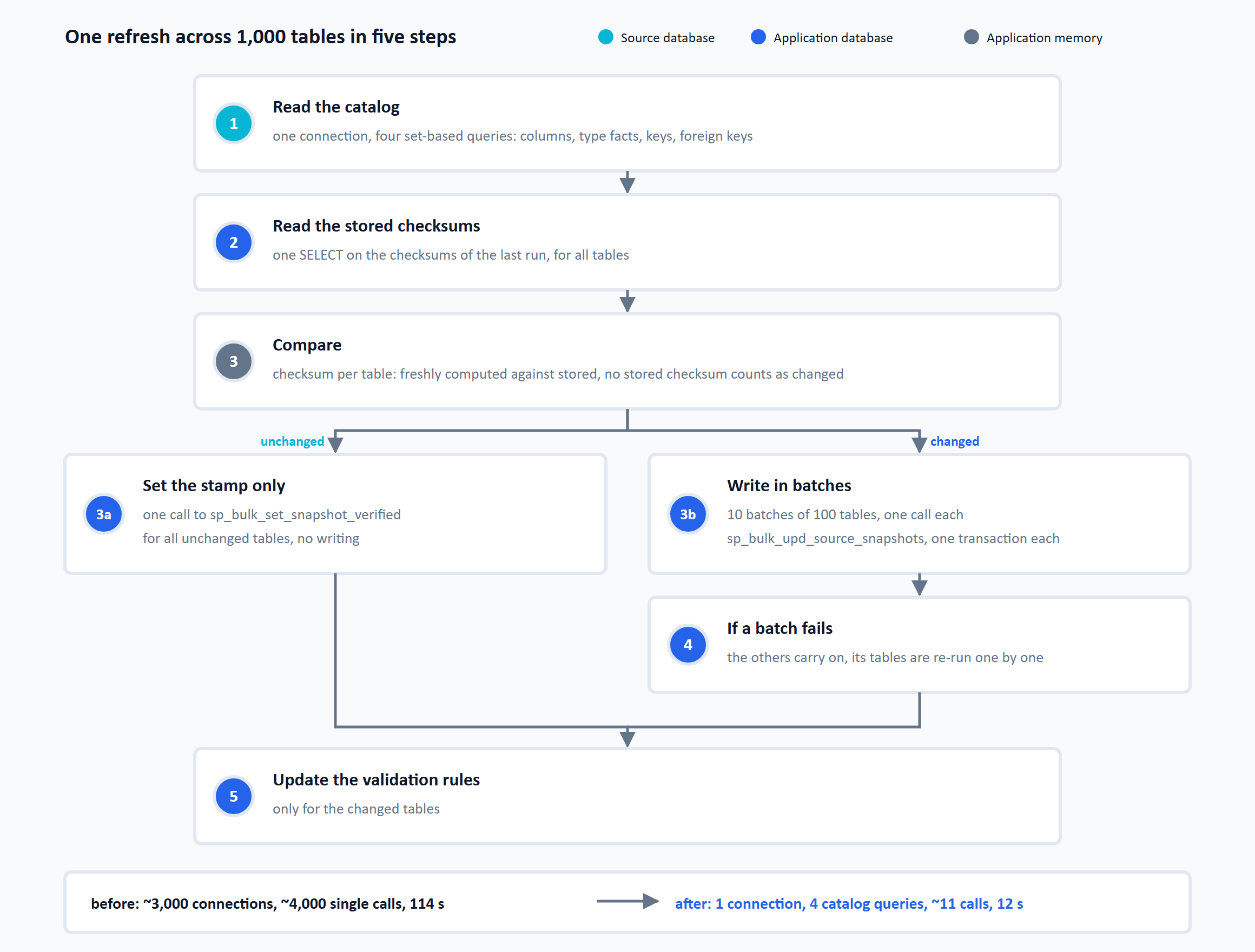
- Read the catalog: The application opens a single connection to the source database and asks four questions, each over all 1,000 tables at once: the columns, the type facts it needs to classify unknown data types, the unique and primary keys, and the foreign keys. After that, the complete catalog sits in the application’s memory. Tables for which the catalog returns not a single column are sorted out here and reported as failed, instead of producing an empty snapshot.
- Read the stored checksums: A single
SELECTon the application’s own database fetches the last stored checksum for all of these tables. That is a different server than in step 1. There the foreign source was queried, here the application’s own data. - Compare: For each table, the application computes a SHA-256 checksum over exactly the data it would store and compares it with the stored one. If no stored checksum exists, the table counts as changed. The result is two groups.
- Unchanged: Nothing is written for these tables. They only receive the stamp “last verified against the source”, through a single procedure call for the whole group.
- Changed: These tables are cut into batches of 100. The number is a constant in the application code and not a setting, and if it does not divide evenly, the last batch is smaller. For each batch, one call goes to the database, with the complete data of the 100 tables as a JSON document in the parameter. The procedure behind it contains no loop of its own. It unpacks the document and writes columns, keys and foreign keys of all tables in the batch with one
DELETEand oneINSERTeach. Every batch is a transaction of its own. For 1,000 changed tables, that is ten calls.
- Catch errors: If a batch fails, the others carry on. The tables of the failed batch are then re-run one by one, through the same path with a set of one element. Only if the error would hit every further call anyway, for instance because the data model has meanwhile been frozen or the connection has been deleted, does the run abort instead of trying again for every single table.
- Update the validation rules: Finally, the validation rules derived from keys are updated, and only for the tables in the “changed” group.
From 3,000 connection setups and 4,000 single calls, this leaves one connection, four catalog queries and roughly ten to eleven procedure calls.
How the New Solution Brings Back the Loop’s Strengths
Of the six strengths from the section “What Spoke for the Loop”, the new solution had to rebuild two explicitly. For the others, the balance is mixed.
Per-table atomicity comes back through the batches. Every batch runs in a transaction of its own, and because the boundary between two batches always lies between two tables and never in the middle of one, no half snapshot of a table comes about even under concurrency. A batch does, however, hold its locks longer than the many small transactions of the loop. So that two overlapping runs do not end up in a deadlock, with each waiting for rows the other holds, the procedure locks the table entries of a batch at the start in a fixed order, with SELECT … ORDER BY id FOR UPDATE. The second run still has to wait until the first one’s batch is complete, and it then works on that state.
Per-table error isolation comes back as a fallback level, as step 4 of the process shows: if a batch fails, the others carry on, and its tables are re-run one by one, so that in the end the count is per table again. The first version did not distinguish two cases here. It treated a single faulty table the same as a cause that hits all tables, such as a connection that has meanwhile been locked. In that case all ten batches failed, and the re-runs produced another 1,000 calls that failed just the same. The finished version recognizes such errors by their message and aborts the re-run.
The constant memory footprint is changed, not preserved. After step 1, the catalog of all tables sits completely in the application’s memory, whereas the loop never held more than one table. What is bounded instead is the size of a single write call: the 100 tables per batch are the result of a trade-off between the size of the document passed in, the duration of the transaction and the time a batch holds locks. A particularly wide table merely makes its batch larger.
Reuse and readability the new solution has given up. The function for a single table no longer exists, and the set-based path is more code, spread across three engines. The inconspicuousness at small scale is preserved but turns out weaker than hoped: 48 tables now take 2.9 to 4.4 seconds instead of an extrapolated five to six. The largest part of that is a fixed base cost, which the results section breaks down.
Skipping Unchanged Tables
For each table, the application computes a checksum over exactly the data it would store and compares it with the checksum of the last run. If both match, the table is not rewritten. It only receives a stamp with the time of the check, so that it stays visible that it was verified against the source.
Set-Based Is Not Automatically Fast: Why a Query Over All Tables Can Be Slower
The first set-based version read the keys of all tables through the two standard views information_schema.table_constraints and information_schema.key_column_usage. That is the portable version over the standard views, and filtered to a single table it had run in the project for years without attracting attention:
  1: SELECT
  2:     T01.table_name
  3:    ,T01.constraint_name
  4:    ,T01.constraint_type
  5:    ,T02.column_name
  6:    ,T02.ordinal_position
  7: FROM
  8:    information_schema.table_constraints T01
  9:    INNER JOIN information_schema.key_column_usage T02
 10:    ON
 11:          T02.constraint_schema = T01.constraint_schema
 12:      AND T02.constraint_name   = T01.constraint_name
 13:      AND T02.table_name        = T01.table_name
 14: WHERE
 15:        T01.table_schema    = 'perf'
 16:    AND T01.constraint_type IN ('PRIMARY KEY', 'UNIQUE')
 17: ORDER BY
 18:     T01.table_name
 19:    ,T01.constraint_name
 20:    ,T02.ordinal_position;
The join runs over schema and constraint name and additionally over the table name in line 13. That condition is necessary because in Postgres a foreign key may carry the same name as the unique constraint of another table in the same schema. Without it, key_column_usage would attribute the columns of that foreign key to the key. Between primary and unique keys the case cannot occur, because the index behind them claims the name within the schema.
Before deployment, the query was measured on Postgres 17. For 1,000 tables it took 4.7 to 5.1 seconds. The same query, issued for each table individually, came to 0.35 to 0.51 seconds extrapolated from a sample of 25 tables. The set-based query was thus around ten times slower than the single queries it was meant to replace, and it would have used up the gain of the entire catalog read.
EXPLAIN ANALYZE showed why. Both views are themselves queries over several system tables, with privilege checks and type conversions. The planner, that is, the part of Postgres that chooses the execution path for every query, had chosen a Nested Loop for this query, a join that walks through the other side again for every row of one side. In this plan, the join condition sat on the Nested Loop itself and not inside the subplan of the view key_column_usage, and so it executed that subplan 1,000 times, once per constraint, which for 1,000 tables with one primary key each means once per table, and each time it read the entire system table pg_constraint. In the plan, that shows up as loops=1000 on exactly this subplan. The timings on such a node are averages per iteration and have to be multiplied by the loops= value, otherwise the most expensive node in the plan looks harmless. So the loop had not disappeared from this plan, it had moved from the application code into the execution plan. As a cross-check, SET enable_nestloop = off brought the same query down from 4.7 seconds to 48 milliseconds. That is a diagnosis and not a solution for production. It does not prove that a Nested Loop would be wrong in principle, only that the chosen plan was expensive for these data volumes.
The rebuild for this article confirms the behavior and at the same time shows that it depends on the version. On Postgres 17.10 the query took 3.9 to 4.8 seconds, on Postgres 18.6 only 29 to 34 milliseconds, because the planner chooses a Hash Join there. That is no blank check for information_schema, though, because a join of the columns view with information_schema.tables ran into the same pattern on 18.6 as well and took over 99 seconds. That is why the procedure in the previous section does without that join.
The solution in the project was a query directly on pg_catalog, the Postgres system tables from which the information_schema views themselves read. It connects pg_constraint through the column array conkey with pg_attribute and, like the view version, restricts itself to primary and unique keys:
  1: SELECT
  2:     T02.relname                       AS table_name
  3:    ,T01.conname                       AS constraint_name
  4:    ,T01.contype = 'p'                 AS is_primary_key
  5:    ,T04.attname                       AS column_name
  6:    ,T03.ordinal_position::int         AS ordinal_position
  7: FROM
  8:    pg_catalog.pg_constraint T01
  9:    INNER JOIN pg_catalog.pg_class T02
 10:    ON
 11:      T02.oid = T01.conrelid
 12:    CROSS JOIN LATERAL unnest(T01.conkey) WITH ORDINALITY AS T03 (attnum, ordinal_position)
 13:    INNER JOIN pg_catalog.pg_attribute T04
 14:    ON
 15:          T04.attrelid = T01.conrelid
 16:      AND T04.attnum   = T03.attnum
 17: WHERE
 18:        T02.relnamespace = 'perf'::regnamespace
 19:    AND T01.contype      IN ('p', 'u')
 20:    -- visibility as in information_schema.columns
 21:    AND (
 22:           pg_has_role(T02.relowner, 'USAGE')
 23:        OR has_column_privilege(T02.oid, T04.attnum, 'SELECT, INSERT, UPDATE, REFERENCES')
 24:        )
 25: ORDER BY
 26:     T02.relname
 27:    ,T01.conname
 28:    ,T03.ordinal_position;
The condition in lines 20 to 24 belongs to the next section. The query returned the same rows, the comparison with EXCEPT ALL showed no difference, and the runtime dropped in a direct comparison run from 4.0 seconds to 13.6 milliseconds. In the rebuild it took around 30 to 60 milliseconds on both Postgres versions. Whoever joins catalog views should therefore look at the execution plan before taking the set-based version for the faster one. The telltale sign is a subplan that reads an entire system table and carries a loops= value equal to the number of rows on the outer side, here the number of tables. The high loops= value alone is not yet a finding, because a Nested Loop that hits an index on the inner side is often the fastest plan. The query on pg_catalog applies only to Postgres. For SQL Server and MySQL, the project has its own catalog queries anyway, there through the sys views and through information_schema respectively, and the problem did not occur there: on both engines, the set-based version was faster than the single queries from the start.
The Privilege Trap When Switching to pg_catalog
The switch to pg_catalog has a side effect worth knowing. information_schema.table_constraints shows only tables that the current role owns or on which it has some privilege other than SELECT. A pure read-only role sees not a single key there, while information_schema.columns shows it all columns. The source connections in the project work with exactly such read-only roles, and that is why the key snapshots of all Postgres sample connections had been empty from the start. Nobody had noticed, because an empty list does not look like an error. The rebuild fixed this defect as a side effect.
pg_catalog has the opposite problem: the system tables pg_constraint and pg_attribute do not filter by the role’s privileges. A role therefore sees the constraint definitions there even for tables whose data it is not allowed to read. That is why the new query carries, in lines 20 to 24, a condition of its own that reproduces the visibility rule of information_schema.columns, and it did not become measurably slower for it. It takes only the privilege check from that view. The view’s remaining filters, such as those against dropped columns or temporary schemas of other sessions, the key query does not need, because a key cannot contain a dropped column and the schema is fixed in advance. So the condition is not a general replacement for the visibility logic of information_schema, and whoever rebuilds a different catalog view on pg_catalog has to carry over its conditions one by one. Whoever derives validation rules from keys, as the article Deriving Data Quality Rules from the Schema describes, should know which role the query runs under.
A second finding belongs to the set-based read itself. The catalog reader creates an entry for every requested table. If the query returns no row for a table, because it no longer exists or the role is not allowed to see its columns, that entry stays empty, without any error message. The code would have turned that into a snapshot without columns and, during reconciliation, deleted the derived validation rules of that table. The code analysis before deployment found this. In a set, a missing element does not stand out, and whoever reads a set therefore has to check for themselves whether something is missing.
The Result: Factor 9 to 19, Targets Still Missed
The measurement after deployment ran on the same server and against the same source database with 1,000 tables:
| Scenario | Before | After | Target |
|---|---|---|---|
| 1,000 tables, all rewritten | 114.4 s, timeout after 60 s | 12.1 s | under 10 s |
| 1,000 tables, unchanged | – | 5.8 to 6.4 s | under 3 s |
| 48 tables, all rewritten | extrapolated 5 to 6 s | 4.4 s | under 2 s |
| 48 tables, unchanged | – | 2.9 to 3.1 s | under 2 s |
| Idle, no stored tables | – | 2.7 s | – |
Instead of 3,000 connections and 4,000 single calls, the refresh now makes three to four catalog queries over a single connection and about ten batch calls. The run with a full rewrite is around nine times faster than before, the run over an unchanged set of tables around 19 times, where this factor measures both changes together, the set-based processing and the skipping of unchanged tables. No run reaches the timeout anymore, and in all nine measurement runs not a single snapshot failed.
All three targets were still missed. The budget estimate before the rebuild had predicted 0.5 to 1.5 seconds for the unchanged run and 2.5 to 5 seconds for the full rewrite. The explanation is in the last row of the table. A refresh over a connection without stored tables reads only the table list and writes nothing, and it still takes 2.7 seconds. That is the fixed base cost of every call to the application server. It covers, among other things, authentication and permission checks, reading the table selection twice, before and after writing, and preparing the response, on a machine that shares its memory with other services. Only the sum was measured, the shares were not recorded individually. On top of this base, the new logic adds around 3.7 milliseconds per table in the unchanged run, across 1,000 tables therefore 3.7 seconds. Both parts together give the upper end of the measured 5.8 to 6.4 seconds (2.7 + 3.7). The base is a lower bound taken from the idle run, because reading the table selection grows with the number of tables. A run that rewrites all 1,000 tables takes more per table than these 3.7 milliseconds, because it additionally deletes and re-inserts 50,000 rows.
Before this explanation was allowed to stand, an obvious alternative was ruled out. Two gigabytes were sitting in swap on the machine. Swap was cleared and the measurement repeated, with practically the same result. That largely ruled out swap as the cause, while other influences of the shared machine remained open. That swap on this same server had once before been the cause of a sluggish application is described in the article The Agent Measures Where I Click. The shared server itself is introduced in the article One VPS, Four Environments, No Cookie Banner.
As long as the loop took 114 seconds, 2.7 seconds of base cost made up a good two percent of the runtime, and nobody noticed them. After the rebuild, in the unchanged run, they are a good 40 percent. Whoever removes the cost per element exposes the fixed costs, and a budget calculation should therefore include them from the start. Lowering the base further would have meant work outside the snapshot code. The decision was to document the deviation and not to optimize further, because the actual problem was gone: there are no more runs lasting minutes, no timeout and no piled-up clicks.
When an Optimization Changes What a Display Means
Skipping unchanged tables has two consequences that have nothing to do with speed.
The first concerns the timestamp. Every snapshot row carries the time at which it was written, and the table register derives a table’s “as of” date from it. As long as every refresh rewrote every table, that moment was also the moment of the last check against the source, because both happened at the same instant. With skipping, the two come apart. An example: a table was last rewritten three weeks ago and has not changed in the source since. Today’s refresh checks it, finds it unchanged and skips it. Its snapshot rows therefore keep the timestamp from three weeks ago. If the register kept showing that timestamp as the “as of” date, a table that was checked a minute ago would display a three-week-old date, and the user would have to assume the refresh had passed it over. That is why there have been two points in time since the rebuild. The snapshot timestamp now moves only when something has actually changed at the source, and so it becomes the change date. The time of the last check is written by the refresh as a stamp of its own, also for every skipped table.
The second concerns the success message. Before, it reported how many snapshots had been updated, and with 1,000 tables it always said 1,000. After the rebuild, “nothing changed” is the normal case, the number of rewritten tables is then zero, and the existing message would have shown “no changes”. The most expensive kind of check, in which 1,000 tables are verified live against the source, would thus have produced exactly the same message as a run over an empty connection. The message therefore states both numbers, that is, how many tables stayed unchanged and how many were rewritten.
Whoever replaces a loop with set-based statements and skips work in the process should also check the displays and messages that rely on the old behavior. Otherwise “a lot was checked” silently turns into “nothing was found”, and the user loses exactly the confirmation they clicked for.
What Remains
- An iteration costs its work plus everything it additionally crosses. Inside the database, an iteration cost around three milliseconds, across connection and application 114. The useful question is therefore not whether a loop is allowed, but what every iteration pays beyond the actual work and how often it runs.
- The budget per element comes before any optimization. Three milliseconds per table settled connection reuse as the sole solution before anyone built it. The budget has to include the fixed costs, otherwise it misses the target in a place where nobody is looking.
- After the rebuild, the execution plan goes on the table. The first set-based query was slower than the single queries because the planner executed it as a Nested Loop over an entire system table. A
loops=value equal to the number of outer rows is the cue to look at the affected subplan, and it gets expensive when that subplan reads an entire system table on every iteration. - An equivalence proof also finds errors in the old code. The comparison before and after the rebuild uncovered a privilege gap through which empty key snapshots had been stored for years.
- Skipped work changes what displays mean. Timestamp and success message had to be redefined, although nothing in their code had changed.
FAQ
No. Set-based means the same as set-oriented: one statement over all rows instead of processing them row by row. It is often faster, because the database can plan the work over the whole set together and fewer fixed costs are incurred per element, but that is no guarantee. How large the gap is depends on what an iteration costs. Inside the database, the loop in the rebuild was around five times slower, and with a few dozen elements that hardly matters. It gets considerably more expensive when every iteration brings its own connection, transaction or network call. If the planner chooses a plan for the set-based statement that internally executes it element by element again, it is even slower than the loop, as the case study shows.
Both process a set element by element and differ in how many system boundaries each element crosses along the way. With the N+1 problem, an ORM first loads a list and then issues a separate query for every element, each of them a separate trip to the database. A cursor loop in a procedure, by contrast, repeats the work inside the database, without additional queries from outside. The case study shows a third variant, in which application code even opens a new connection per element. Every boundary between the loop and the data, that is, a connection, a process or a transaction, raises the fixed cost of an iteration.
information_schema views sometimes so slow? The views in information_schema are themselves queries over several system tables. If you join two of them, it can happen that the Postgres query planner cannot push the join condition into the views and evaluates one view completely for every row of the other. In the execution plan you recognize this by a Nested Loop whose inner subplan reads an entire system table and carries a loops= value equal to the number of outer rows, here the number of tables. Whether it happens depends on the query and the version: the key query was affected on Postgres 17 and not on Postgres 18, the join of columns and tables was affected on both. The remedy is a query directly on pg_catalog or a single view without a join.
information_schema.table_constraints? This view shows only tables that the role owns or on which it has some privilege other than SELECT. information_schema.columns, by contrast, shows the columns already with SELECT. A role that may only SELECT on a table therefore sees all of its columns but none of its primary or unique keys. Whoever needs the keys for such a role reads them from pg_constraint and checks visibility themselves. The query in the case study reproduces the rule of information_schema.columns and not that of table_constraints: it shows a role the keys if the role owns the table, checked with pg_has_role, or has a privilege on the column, checked with has_column_privilege.
The COMMIT alone is not enough for that. It secures what has already been written, but it still ends the call at the first unhandled error. The loop can only keep running if every iteration gets its own BEGIN … EXCEPTION block that catches the error and increments a counter. When the block catches an error, Postgres has already rolled back the changes of that iteration, because a block with error handling runs as a subtransaction. The COMMIT after it then has nothing left to commit for that table, and no half snapshot can come about. There is a trap here: the COMMIT has to go after this block, not inside it. Inside a block with error handling it fails with cannot commit while a subtransaction is active, and a WHEN OTHERS handler swallows exactly this error silently. The procedure then runs through without error and writes nothing.
The duration can be read from the written data. If every iteration writes its rows in a transaction of its own and stamps them with now(), the span between the smallest and the largest timestamp after an undisturbed run gives the duration of the loop up to the last iteration. If everything runs in a single transaction, now() returns the same value everywhere, and the column then needs clock_timestamp() as its default. In the long run this is no substitute for instrumentation, but it works after the fact and without any code change.
Related Articles
Downstream:
- Design Pattern // The Architecture of an ETL Process — at which stage of an ETL pipeline catalog reads like this one have their place.
- Deriving Data Quality Rules from the Schema — how mandatory fields, keys and type limits from
information_schematurn into validation rules. - Reading Complex XML in SQL Server — Shredding a Thousand Attributes Generically Instead of Looping for Hours — the same idea applied to an XML document: shred generically instead of looping per object type and attribute.
From the same project:
- The Agent Measures Where I Click — four debugging sessions in which a measurement replaced the guess.
- One VPS, Four Environments, No Cookie Banner — the shared machine on which these measurements ran as well.
- Agentic Coding from a User’s Perspective — how working with a coding agent changes the daily routine.